|
|
The descriptive geometry is the discipline to study the methods of three-dimentional objects mapping to the plane and also the graphical methods for positional and measuring solutions by the means of their planar object's images (models). |
|
| |
Part one. The Modeling of Geometry Objects |
| |
Point is the most simple object of three-dimentional space. All points are classified as intrinsic points and nonintrinsic points (positioned in infinity). We shall mark nonintrinsic point on the model with an arrow, that defines the direction to this point. All other objects of three-dimentional space are possible to understand as the geometrical holders of three-dimentional points. We shall use the projection procedure in order to distribute all of the volumetrical objects by the means of planar schemes and drawings. |
|
| |
|
| |
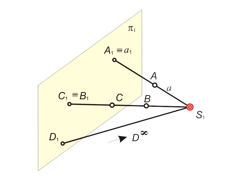
Let's select a three-dimentional point S1 – the center of projection and a plane π1 – the plane of projections (fig. 1.1). The center S1 and a plane of projections π1 represents themselves as apparatus of projection. In order to determine the projection of arbitrary point А of initial space we shall pass over the next steps:
1. Draw the straight line a over the center S1 and point А;
2. Define the point of crossing the line a with the plane π1: A1=a ∩ π1.
Th got poin A1 is called as projection of point A (image of A) to the plane π1 from the center S1. All other projections of other points could be defined the same way. The straight line a, that pass over the center S1 is called as projective line. It maps to the projection plane as a point. The projection are classied as central or parallel correspondently to disposition of the center S1 - intrinsic or nonintrinsic.
When the point S1 is a intrinsic point of a space, we've got an apparatus of central projection (fig. 1.1). The central projection supposes, that the projection of initially nonintrinsic point D∞ could be intrinsic point D1.
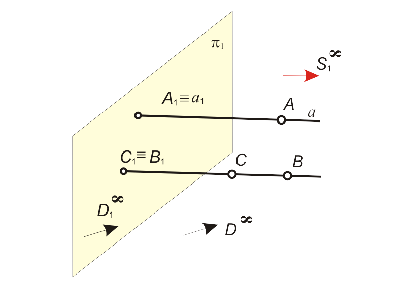
When the central point is in an infinity S1, we've got an apparatus of parallel projection (fig. 1.2). The central projection supposes, that the projection of initially nonintrinsic point D∞ is allways nonintrinsic point D1∞. When the direction of parallel projecting is not rectangular with the plane π1 (an angle φ≠90°), we've got an apparatus of bevel projection.
In the special case of parallel projecting, when the angle φ=90° (projection lines are perpendicular to th plane of projections ), we've got an apparatus of rectangular (orthogonal) projection. |
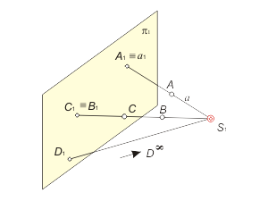
Fig. 1.1
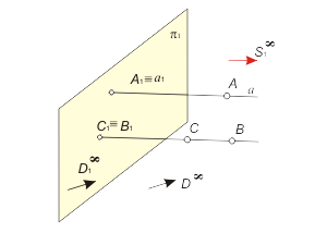
Fig. 1.2 |
| |
The Properties of Parallel Projecting |
| |
1. The image of a point is a point.
2. The image of a line is a line. Only the image of a projective line is a point.
3. The points and lines while projecting keep their incidence. It means, that images of crossing lines intersect each other by the point, which is the image of the crossing point of initial lines.
4. The image of parallel lines are parallel to each other too.
5. The length ratio of two parallel straight segments is equal to the ratio of length of initial segments.
6. The parallel projection of planar figure, that is coincidental to the plane, parallel to the plane of projection, is congruent (equal) to initial figure.
The models, got as the result of central or parallel projecting, are irreversible. The multitude of points, coincidental to the projective line a, corresponds a single point A1 on a plane. It means, that a single projection of an object on the plane π1 corresponds to multitude of objects in three-dimensional space. In order to get a reversible model, that supports the ablity to reconstruct the shape, dimensions and position of an object in a space, ones use the method of two images. |
|
| |
The Method of Gaspard Monge |
| |
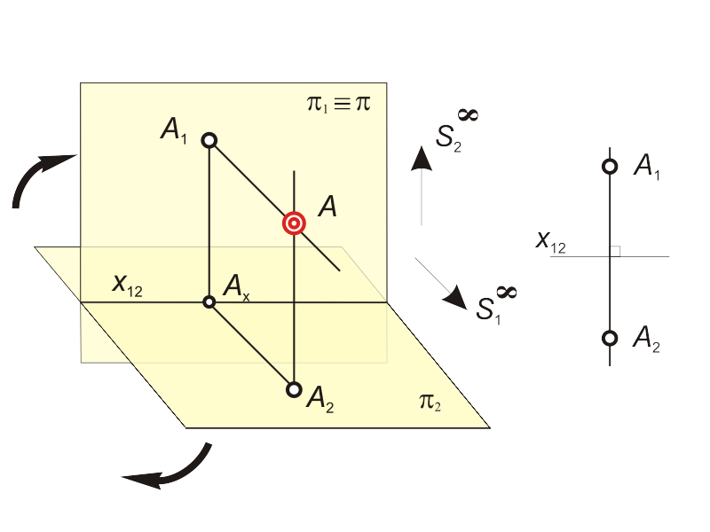
The French Mathematician Gaspard Monge (1746 - 1818) have got an idea to represent the mapping of volumetrical objects, using rectangular projecting to the pair mutualy perpendicular planes. Let's get in the three-dimentional space two mutualy perpendicular planes – π1 ⊥ π2. The plane π1 is named as frontal plane of projections, and π2 as horizontal plane of projections. The projecting to the planes π1 and π2 from the corresponding centers S1∞ and S2∞ is rectangular (fig. 1.3) In order to get a planar model, we shall turn the plane π2 over axis x12 till its coincidence with the plane π1. |
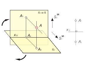
Fig. 1.3
|
| |
|
| |
The model of three-dimensional point А on the distribution diagram of Monge corresponds to the pair of planar points А1 and А2, both icident to linkage line, which spreads perpendicular direction to an axis x12.
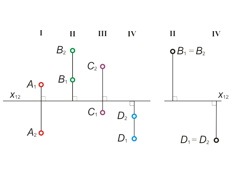
Let's consider possible distribution of points projection on a diagram of Monge in relation to an axis x12 in dependence of initial three-dimensional points distribution, comparatively to position of projectional planes π1 and π2 placement. As it shown on fig. 1.4, points А, В, С, D are distributed on I, II, III и IV quarters of space. The possible variants of their projective images placement are shown at Monge diagram (fig. 1.5) in correspondance to an axis x12. |
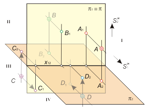
Fig. 1.4
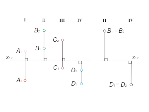
Fig. 1.5 |
| |
|
| |
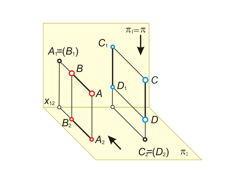
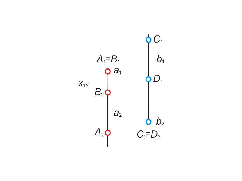
The two points, that are coincidental to one projective line, are known as concurrent. It is possible to estimate the mutual visibility of geometrical objects, using the concurrent points by the means of Monge diagram.
Fig 1.6 distributes the two pairs of concurrent points A, B (АВ ⊥ π1) and C, D (CD ⊥ π2 ). It is shown with an arrows the direction of observer's sight. The point meants visible, if it is closer to the observer. While projecting to the plane π1 the point A is visible, and while projecting to the plane π2 – the point С is visible. |
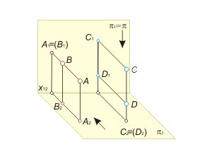
Fig. 1.6 |
| |
The Modeling of Descartes Rectangular Coordinate System |
| |
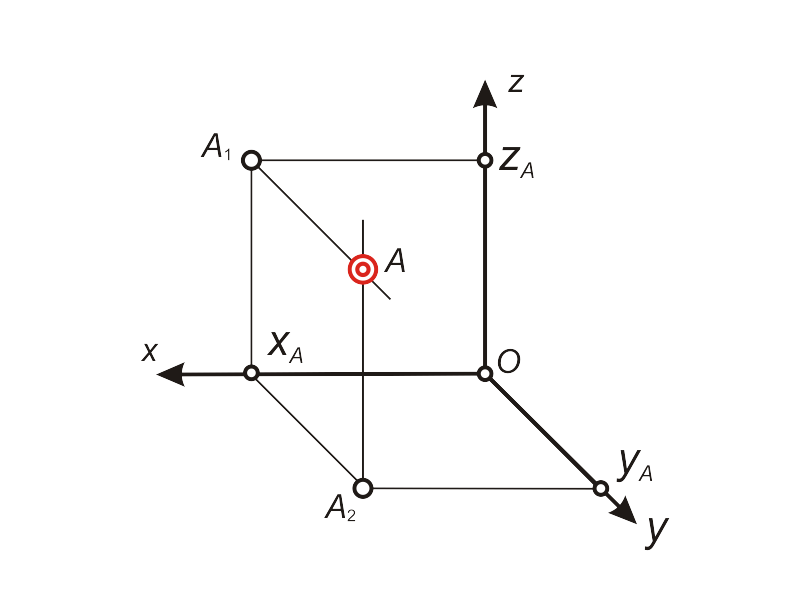
In order to definition of point's placement in three-dimentional space we shall use the rectangular Descartes coordinate system (xyz), which represents itself as three mutually perpendicular axis (fig. 1.7). |
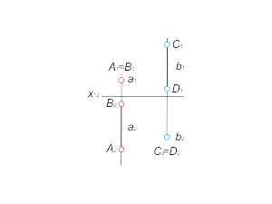
Fig. 1.7 |
According to this system the point A is declared with the coordinates (xA, yA, zA). The coordinates of a point could be positive or negative, as well.
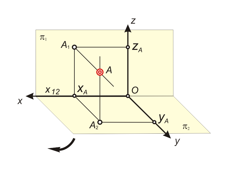
In order to model the coordinate system by the means of Monge diagram we shall pass over the next set of operations:
- combine the coordinate plane xOz with the frontal plane of projections π1 and combine the coordinate plane xOy with the horizontal plane of projections π2 (fig. 1.8);
- pass to one single plane (to Monge diagram).
The projections of coordinate axis x, y, z and images of point А are shown at fig. 1.9. |
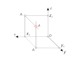
Fig. 1.8
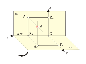
Fig. 1.9 |
Obviously, that the frontal projection А1 of the point А, would be defined with coordinates (xA, zA), but the horizontal projection А2 – with coordinates (xA, yA).
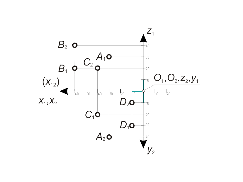
We shall mark positive values (xA, yA, zA) from the point O(О1, О2) to the left, down and up on the projections x1, y2 и z1 correspondently, negative values (xA, yA, zA) - from the point O(О1,О2) to the right, up and down on the projections x2, y2 и z1 correspondently. Fig. 1.10 presents the points А, В, С, D with coordinates: А(30, 40, 30); В(60, -40, 20); С(40, -20, -20); D(10, 10, -30). |
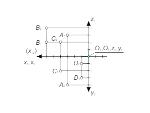
Fig. 1.10 |
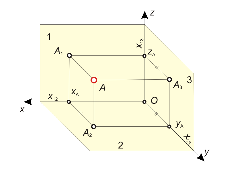
As it already known, two projections of a point completly define its space distribution. However, while getting the solutions of descriptive geometry tasks and while technical drawing ones oftenly use the profile plane π3(π1 ⊥ π3 ⊥ π2).
While modeling the rectangular coordinate system, we shall combine the plane π3 with coordinate plane (yOz) (fig. 1.11), then profile projection А3 of the point А would be defined with coordinates (yA, zA). Passing by the planar model, we shall rotate the plane π3 around an axis x13 till its coincidence with the plane π1. |
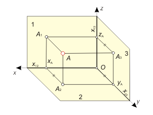
Fig. 1.11 |
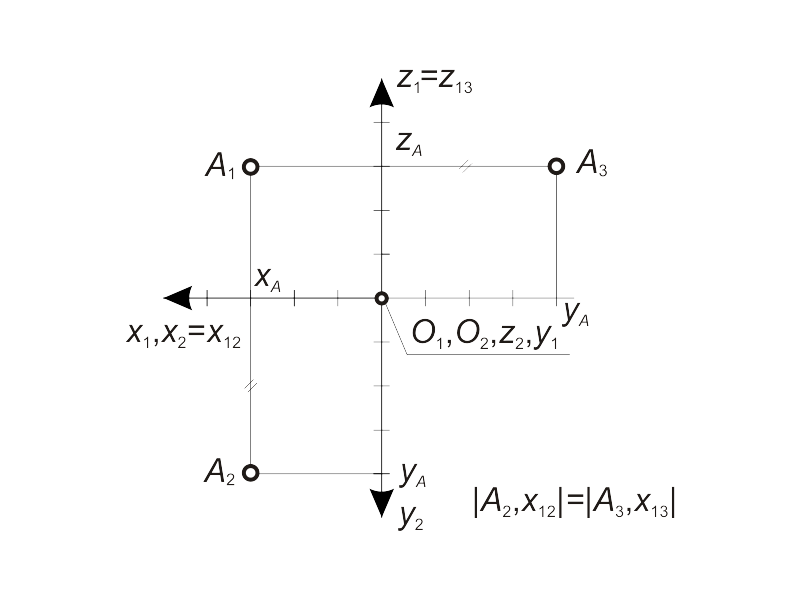
Because of community of coordinate zA for projections А3 and А1 and coordinate yA – for А3 and А2, the placement of projection А3 at planar model it is possible to define, like the next set of operations:
- draw a straight line (linkage line) in perpendicularity to line z1(x13) (fig. 1.12);
- measure the distance between the projection А2 and an axis x12 and put aside its value along the linkage line from the axis x13. |
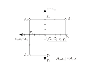
Fig. 1.12 |
| |
| |
|
|
|